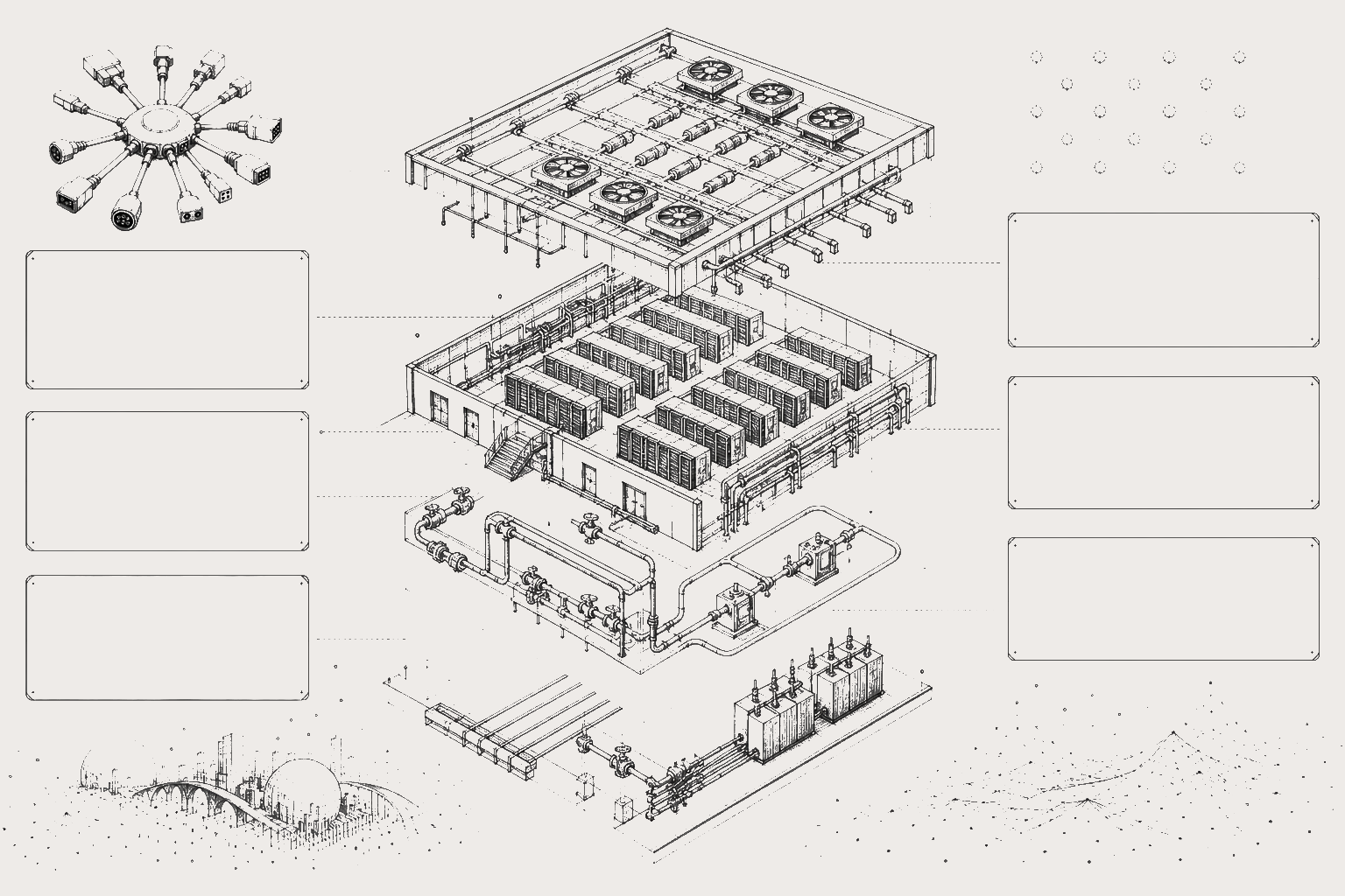
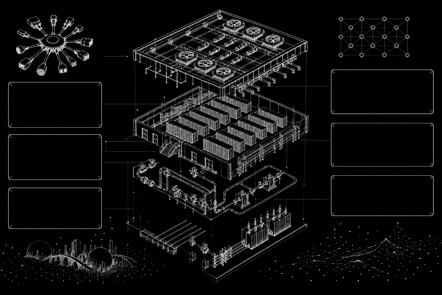
MECE Framework for Data Center Architecture
A MECE (Mutually Exclusive, Collectively Exhaustive) decomposition rooted in physical-scale progression — drilling from the macro campus level (kilometer-scale) down to micro-components (millimeter-scale). Each layer has well-defined input/output boundaries, and each maps to a distinct investment thesis and due-diligence focus area.
Framework Overview
Key Inter-Layer Boundaries
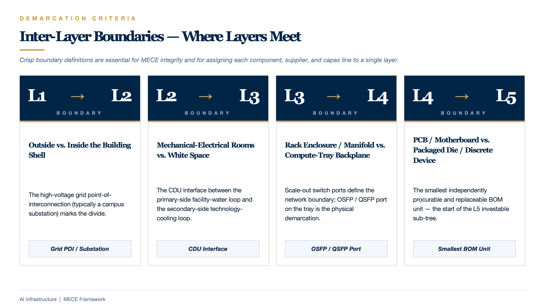
| Boundary | Demarcation Criterion |
|---|---|
| L1 / L2 | Outside vs. inside the building shell; the high-voltage grid point-of-interconnection (typically a campus substation) marks the divide |
| L2 / L3 | Mechanical/electrical rooms vs. white space; the CDU interface between the primary-side facility-water loop and the secondary-side technology-cooling loop |
| L3 / L4 | Rack enclosure / rack manifold vs. compute-tray backplane; Scale-out switch ports define the network boundary |
| L4 / L5 | PCB / motherboard vs. packaged die / discrete device; the smallest independently procurable and replaceable BOM unit |
L1 — Macro Resources & Campus Layer
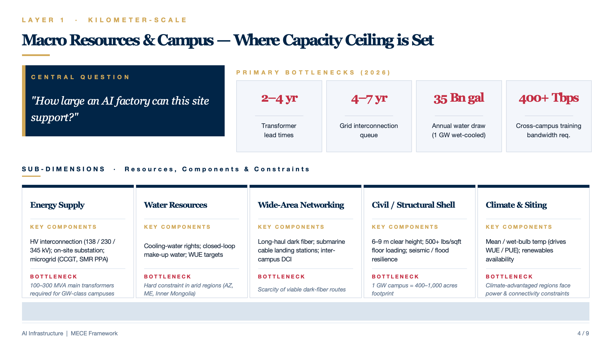
Central question: "How large an AI factory can this site support?"
| Sub-Dimension | Key Components / Resources | Typical Scale | Primary Bottleneck (2026) |
|---|---|---|---|
| Energy Supply | HV grid interconnection (138 / 230 / 345 kV), on-site substation, microgrid (natural-gas CCGT / SMR nuclear PPA) | GW-class campuses require 100–300 MVA main transformers | Transformer lead times of 2–4 years; grid-interconnection queues of 4–7 years |
| Water Resources | Cooling-water rights, closed-loop make-up water, WUE targets | A 1 GW wet-cooled campus consumes ≈ 35 billion gallons per year | Hard constraint in arid regions (Arizona, Middle East, Inner Mongolia) |
| Wide-Area Networking | Long-haul dark fiber, submarine-cable landing stations, inter-campus DCI | Cross-campus training demands > 400 Tbps | Scarcity of viable dark-fiber routes |
| Civil / Structural Shell | 6–9 m clear height, 500+ lbs/sqft floor loading, slab-on-grade, seismic & flood resilience | A 1 GW campus spans 400–1,000 acres | Structural-steel and concrete supply-chain lead times |
| Climate & Siting | Annual mean temperature, wet-bulb temperature (drives WUE / PUE), renewable-energy resource availability | Northern Europe / Pacific Northwest are optimal | Climate-advantaged regions often face power and connectivity constraints |
Key Investment & Due-Diligence Questions:
- Has grid interconnection been secured? Is the Interconnection Service Agreement (ISA) executed?
- Does the site offer expansion optionality (Phase 2 / 3 land reserves)?
- Are water-allocation quotas sufficient? Has the environmental impact assessment been approved?
- Can building specifications accommodate next-generation GPUs (6 m+ clear height, 500+ lbs/sqft floor loading)?
L2 — Facility & Mechanical-Electrical Layer
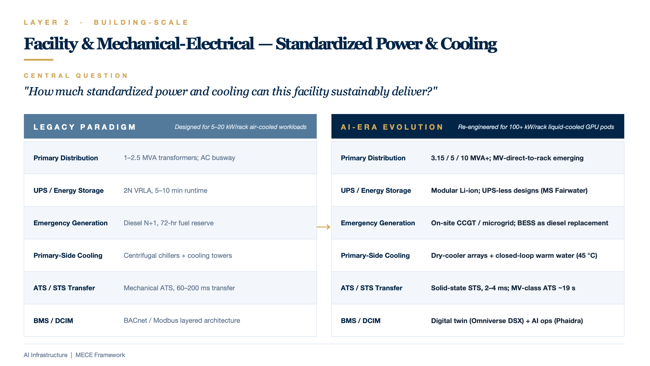
Central question: "How much standardized power and cooling can this facility sustainably deliver?"
| Sub-Dimension | Key Components | Legacy Paradigm | AI-Era Evolution |
|---|---|---|---|
| Primary Distribution Chain | MV switchgear → transformer → LVMS main distribution board | 1–2.5 MVA transformers | 3.15 / 5 / 10 MVA+; emerging trend of MV-direct-to-rack distribution |
| UPS / Energy Storage | Centralized double-conversion UPS, VRLA battery rooms, BESS | 2N VRLA, 5–10 min runtime | Modular lithium-ion; select deployments eliminate UPS entirely (e.g., Microsoft Fairwater) |
| Emergency Generation | Diesel gensets, fuel systems, exhaust routing | Diesel N+1, 72-hour fuel reserve | Natural-gas CCGT / on-site microgrids; BESS as diesel replacement |
| Primary-Side Cooling | Chillers, cooling towers, dry coolers, large-bore piping | Centrifugal chillers + cooling towers | Dry-cooler arrays + closed-loop warm-water systems (45 °C supply); chiller elimination |
| ATS / STS Transfer | Utility-to-generator changeover, UPS-to-bypass transfer | Mechanical ATS, 60–200 ms transfer | Solid-state STS, 2–4 ms transfer; MV-class ATS at ≈ 19 s |
| BMS / DCIM | Building management, environmental monitoring, capacity management | BACnet / Modbus layered architecture | Digital twin (NVIDIA Omniverse DSX) + AI-driven operations (DeepMind, Phaidra) |
Key Investment & Due-Diligence Questions:
- What are the age and lifecycle status of UPS units, gensets, and chillers?
- What is the supply-chain obsolescence / spare-parts risk for critical equipment (PLC controllers, breaker models)?
- Can the cooling infrastructure transition from air-cooled to liquid-cooled (primary-side water temperature, pipe pressure ratings, CDU tie-in points)?
- What is the maturity of the BMS / DCIM stack (AIOps readiness, data-migration complexity post M&A)?
L3 — Cluster & Rack Layer (Pod)
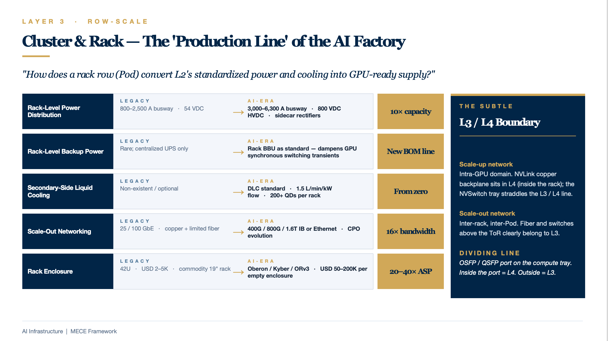
Central question: "How does a rack row (Pod) convert L2's standardized power and cooling into GPU-ready supply?"
| Sub-Dimension | Key Components | Legacy Paradigm | AI-Era Evolution |
|---|---|---|---|
| Rack-Level Power Distribution | Busway, rack PDU, sidecar power shelf | 800–2,500 A busway, 54 VDC | 3,000–6,300 A busway, 800 VDC HVDC, sidecar rectifiers |
| Rack-Level Backup Power | Rack BBU, short-duration energy storage | Rare | Rack BBU as standard (dampens GPU synchronous switching transients) |
| Secondary-Side Liquid Cooling | CDU, manifold, QD (quick-disconnect) fittings, make-up water unit, leak detection | Non-existent / optional | DLC as standard; 1.5 L/min/kW flow rate; 200+ QDs per rack |
| Scale-Out Networking | ToR switch, spine / core switches, fiber tray, MMR | 25 / 100 GbE, copper + limited fiber | 400G / 800G / 1.6T InfiniBand or Ethernet; CPO evolution |
| Rack Enclosure | 19" / 21" rack, doors, cable management | 42U, USD 2–5K | Oberon / Kyber / ORv3 chassis; USD 50–200K per empty enclosure |
The Subtle L3 / L4 Boundary
- Scale-up network (intra-GPU-domain): NVLink copper backplane physically resides in L4 (inside the rack); however, the NVSwitch tray — as a standalone unit — straddles the L3/L4 boundary.
- Scale-out network (inter-rack, inter-Pod): Fiber and switches above the ToR clearly belong to L3.
- Dividing line: The OSFP / QSFP port on the compute tray — inside the port is L4; outside the port is L3.
Key Investment & Due-Diligence Questions:
- Does the busway ampacity support next-generation density (120–600 kW per rack)?
- Does the liquid-cooling system meet the availability requirements of AI training workloads (leak detection, redundancy design)?
- Does Scale-out bandwidth prevent GPU under-utilization (risk of 33% idle loss)?
- Rack compatibility: which of Oberon / ORv3 / Kyber are supported? What is the retrofit cost?
L4 — Node & Server Layer
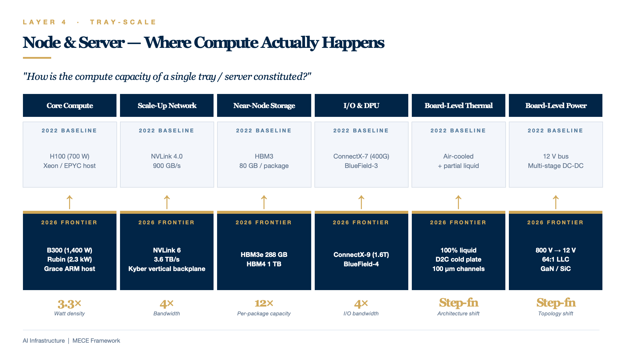
Central question: "How is the compute capacity of a single tray / server constituted?"
| Sub-Dimension | Key Components | 2022 Baseline | 2026 Frontier |
|---|---|---|---|
| Core Compute | GPU / AI accelerator, host CPU | H100 (700 W), Xeon / EPYC | B300 (1,400 W), Rubin (2.3 kW), Grace ARM host |
| Scale-Up Network | NVLink copper backplane, NVSwitch | NVLink 4.0 / 900 GB/s | NVLink 6 / 3.6 TB/s, Kyber vertical backplane |
| Near-Node Storage | HBM (on-package), NVMe SSD, E1.S | HBM3, 80 GB | HBM3e 288 GB, HBM4 1 TB |
| I/O & DPU | SmartNIC, DPU, PCIe bus | ConnectX-7 (400G), BlueField-3 | ConnectX-9 (1.6T), BlueField-4 |
| Board-Level Thermal | Cold plate, heat sink, fans | Air-cooled + partial liquid cooling | D2C cold plate, 100% liquid-cooled, 100 μm micro-channel |
| Board-Level Power | VRM / power IC, on-board BBU | 12 V bus, multi-stage DC-DC | 800 V → 12 V single-stage 64:1 LLC, GaN / SiC devices |
Key Investment & Due-Diligence Questions:
- What is the liquid-cooling readiness of the server tray (full liquid vs. hybrid)?
- What is the NVLink domain size (NVL8 → NVL72 → NVL576)?
- Is HBM supply locked in? What is the hedging mix across SK Hynix / Samsung / Micron?
- What is the OEM certification status of cold plates and quick-disconnect fittings?
L5 — Micro-Component Layer (Vertical Drill-Down)
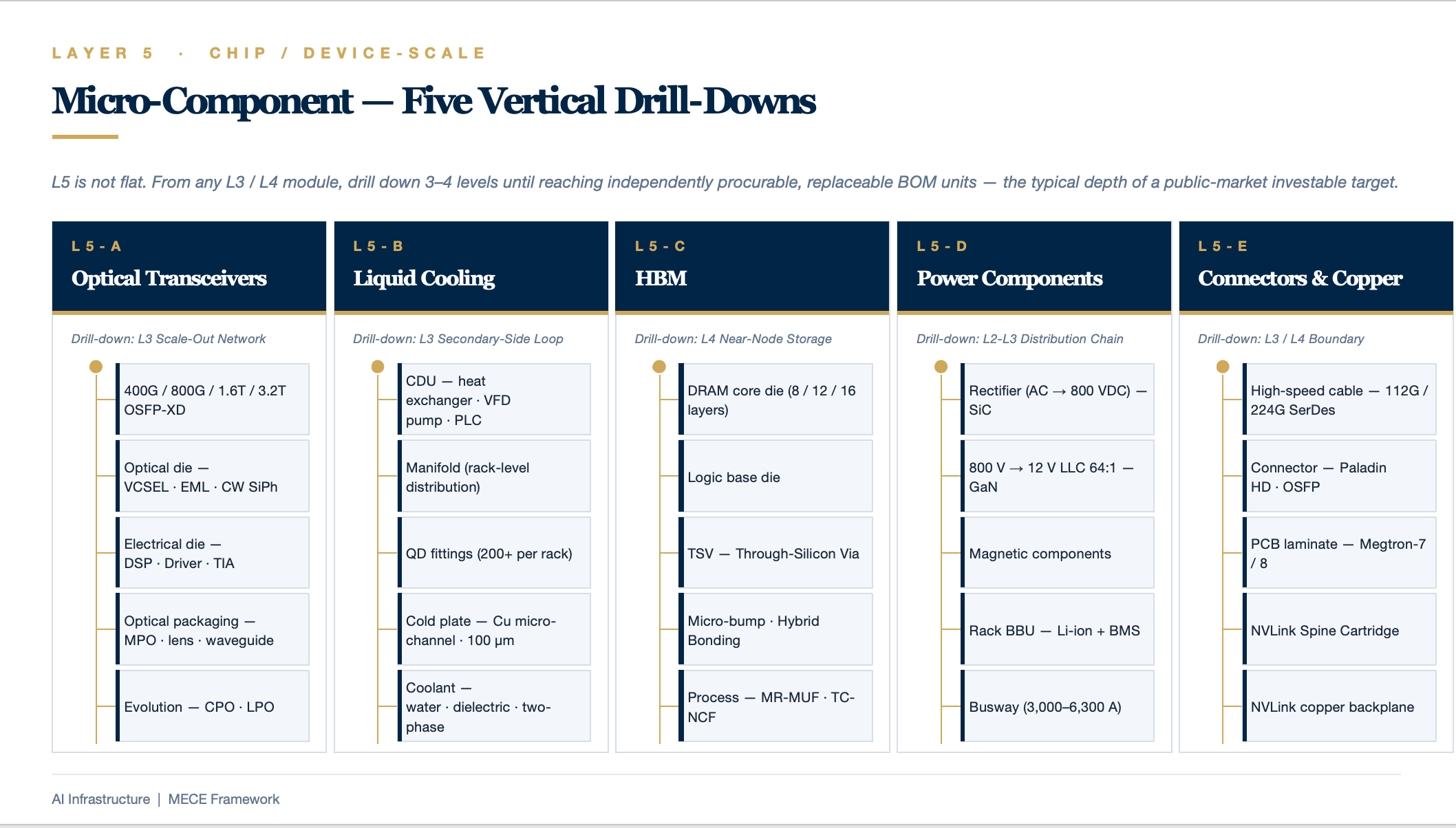
Governing principle: L5 is not a flat layer but rather a sub-tree that can be drilled into from any module in L3 or L4. Stopping rule: Drill down until the level at which an independently investable public-market target exists — typically 3–4 levels deep.
L5-A: Optical Transceivers (Drill-Down from L3 Scale-Out Network)
L3  Scale-Out Network
 └─ L4  Optical Transceiver (400G / 800G / 1.6T / 3.2T OSFP-XD)
       ├─ Optical Die:  Laser (VCSEL / EML / CW SiPh), Photodetector, Modulator
       ├─ Electrical Die:  DSP, Driver, TIA, CDR
       ├─ Optical Packaging:  MPO connector, lens, waveguide
       └─ Evolution:  CPO (Co-Packaged Optics), LPO (Linear-Drive Pluggable Optics)
L5-B: Liquid-Cooling System (Drill-Down from L3 Secondary-Side Cooling)
L3  Secondary-Side Liquid-Cooling Loop
 ├─ CDU (Coolant Distribution Unit)
 │     ├─ Plate heat exchanger
 │     ├─ Variable-frequency pump package
 │     ├─ Sensors / filters / degassing unit
 │     └─ Control PLC
 ├─ Manifold
 ├─ QD Quick-Disconnect Fittings (200+ per rack)
 ├─ Cold Plate
 │     ├─ Copper micro-channel machining (100 μm precision)
 │     ├─ Sealing / anti-corrosion coating
 │     └─ Blind-mate / side-entry structure
 └─ Coolant (treated water, dielectric fluid, two-phase refrigerant)
L5-C: HBM (Drill-Down from L4 Near-Node Storage)
L4  HBM Stack
 ├─ DRAM core die (8 / 12 / 16 layers)
 ├─ Logic base die
 ├─ TSV (Through-Silicon Via)
 ├─ Micro-bump / Hybrid Bonding
 └─ Process:  MR-MUF (SK Hynix), TC-NCF (Samsung)
L5-D: Power Components (Drill-Down from L2–L3 Distribution Chain)
L3  800 VDC Rack Power
 ├─ Rectifier (AC → 800 VDC)
 │     ├─ SiC power devices
 │     └─ Digital control IC
 ├─ 800 V → 12 V LLC Converter (64:1)
 │     ├─ GaN power devices
 │     ├─ Magnetic components
 │     └─ Controller IC
 ├─ Rack BBU
 │     ├─ Li-ion cells (LFP / NMC)
 │     └─ BMS / protection board
 └─ Busway
L5-E: Connectors & Copper Interconnects (Drill-Down from L3/L4 Boundary)
L4  NVLink Copper Backplane  +  L3  Scale-Out Copper Interconnects
 ├─ High-speed copper cable (112G / 224G SerDes)
 ├─ Connector (Paladin HD, high-density OSFP)
 ├─ PCB laminate (Megtron-7 / 8)
 └─ NVLink Spine Cartridge
Electrical Architecture & Power Density Evolution
From Dual-Utility-Feed 2N / 2(N+1) System-Level Redundancy
Utility normal ────────┬─── Utility outage ──────────────────────────→ Time
                       │
                       │ 0 ms ────── 10–30 s ────── Hours ────── Days
                       │   ↑              ↑              ↑
                       │  UPS assumes     Genset starts   Genset sustains
                       │  load seamlessly  and runs until  operations
                       │                   utility returns
- UPS covers 0 seconds to 10–30 seconds. Its mission is to bridge the gap seamlessly — the load perceives zero interruption when the utility drops. However, its batteries last only 5–15 minutes; beyond that, they are depleted.
- Diesel generator covers tens of seconds onward through days. Its mission is long-duration utility substitution.
- Utility feed is the primary power source under normal conditions.
Per Schneider Electric White Paper 75, availability ranks as follows: N (standalone) < isolated redundant < parallel redundant (N+1) < distributed redundant < 2N / 2(N+1) system-level redundant (highest). An N+1 system achieves roughly 99.98–99.99% availability; a 2N system reaches 99.995%+; and a 2(N+1) configuration approaches 99.9999% (six nines). Uptime Institute surveys consistently show that power-related failures top the list of severe / major outage causes, with UPS and distribution faults accounting for roughly 30–40% of all downtime events.
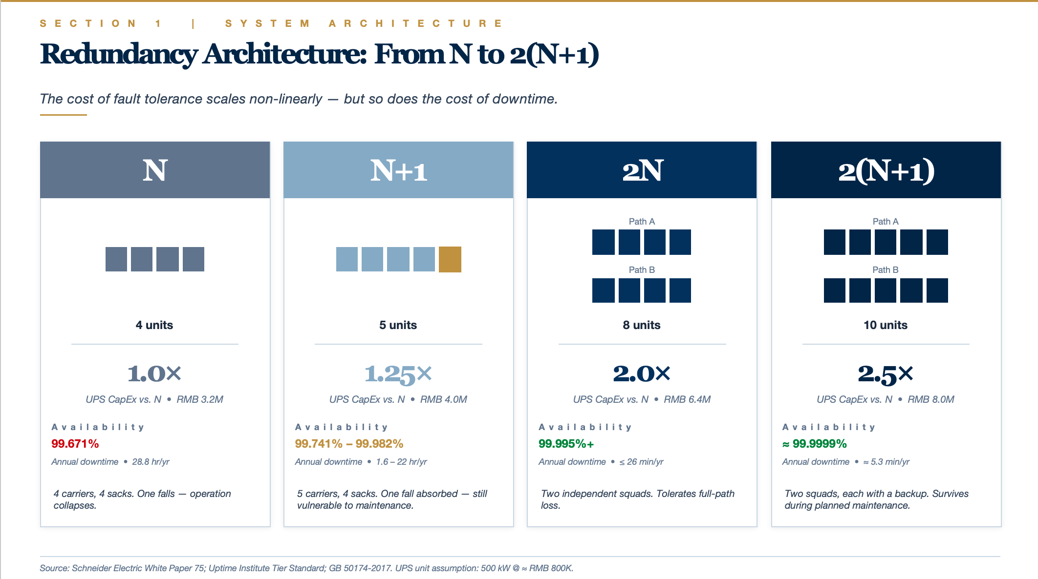
N = the minimum number of units required to serve the full load.
Suppose a facility needs 4 × 500 kW UPS to carry 2 MW of load — then N = 4.
| Tier | Unit Count | Meaning | Analogy |
|---|---|---|---|
| N | 4 | Exactly sufficient; zero redundancy | 4 people carrying 4 sacks of rice — lose one and the whole thing collapses |
| N+1 | 5 | 1 standby unit added | 5 people carrying 4 sacks — one can fall and the team still copes |
| 2N | 4 + 4 = 8 | An entire duplicate system | Two independent squads of 4, mirroring each other |
| 2(N+1) | (4+1) + (4+1) = 10 | Two systems, each with its own +1 spare | Two squads of 5 (each with 1 backup) |
2N: Dual-System Mirroring
Two fully independent power chains (Path A + Path B), each independently capable of carrying 100% of the load.
Utility A → Transformer A → UPS Bank A (4 units) → PDU-A ┐
                                                          ├──→ Dual-corded servers (two PSUs)
Utility B → Transformer B → UPS Bank B (4 units) → PDU-B ┘
- During normal operation, each path carries 50% of the load (leaving 50% headroom per path).
- If an entire path fails — including its utility feed, transformer, UPS bank, and distribution panel — the other path instantly assumes 100%.
- Servers are dual-corded (dual PSUs) and handle the switchover internally.
Key attribute: tolerates full-chain failure, including human error (tripping the wrong A-path breaker), fire, flooding, or any event that renders an entire path inoperable.
2(N+1): Dual-System Mirroring with Per-Path +1 Redundancy
On top of 2N, each path adds one standby UPS internally.
Utility A → Transformer A → UPS Bank A (4+1 = 5 units) → PDU-A ┐
                                                                 ├──→ Dual-corded servers
Utility B → Transformer B → UPS Bank B (4+1 = 5 units) → PDU-B ┘
- If 1 UPS fails within Path A, Path A self-heals internally (the remaining 4 units still carry full load).
- If all of Path A goes down, Path B takes over.
- If 1 UPS fails in Path A and simultaneously 1 UPS fails in Path B, the system remains unaffected.
The Critical Distinction
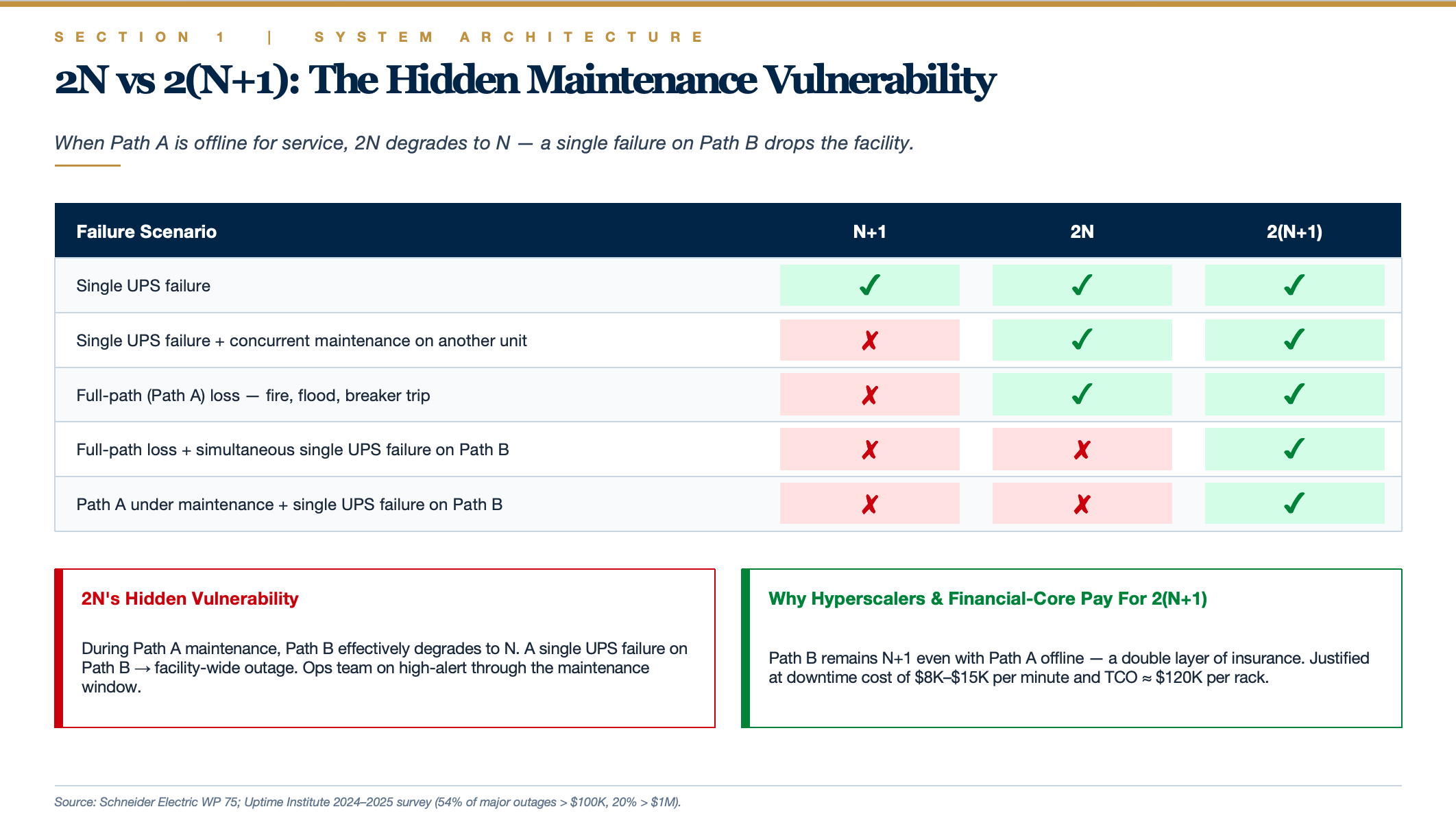
2N's hidden vulnerability: When Path A is taken offline for maintenance, Path B effectively degrades to N (no redundancy). At that point, a single UPS failure on Path B triggers a facility-wide outage.
2(N+1) solves exactly this problem: With Path A offline, Path B still operates as N+1 (redundant) — a double layer of insurance.
Real-world operations example — annual UPS maintenance on Path A:
- 2N system: Path A must be de-energized; Path B now shoulders the entire load with zero redundancy. If any single UPS on Path B fails during the window → full facility outage. The ops team spends the night on high alert.
- 2(N+1) system: Path A de-energized; Path B remains N+1. A single UPS failure on Path B is absorbed internally — the facility is unaffected. The ops team operates with composure.
This is why financial-core data centers and hyperscaler mission-critical clusters typically deploy 2(N+1), while standard enterprise Tier IV facilities consider 2N sufficient.
Cost Perspective
Using a 2 MW facility's UPS as an example (each unit 500 kW, ≈ RMB 800K / ≈ USD 110K):
| Configuration | UPS Count | UPS CapEx | Multiple of N |
|---|---|---|---|
| N | 4 units | RMB 3.2M | 1.0× |
| N+1 | 5 units | RMB 4.0M | 1.25× |
| 2N | 8 units | RMB 6.4M | 2.0× |
| 2(N+1) | 10 units | RMB 8.0M | 2.5× |
Note: This covers UPS hardware alone. Switchgear, batteries, floor space, and cooling must also scale accordingly, so total 2N investment runs roughly 2.2–2.5× that of N, and 2(N+1) roughly 2.7–3×.
Standards & Availability Benchmarks
China's GB 50174-2017 (Code for Design of Data Centers) classifies facilities into Grades A, B, and C. Grade A (fault-tolerant) requires dual utility feeds, 2N-redundant architecture, diesel-generator backup, and UPS battery runtime of no less than 15 minutes. Grade B (redundant) recommends dual utility feeds with N+1 UPS redundancy. Grade C (basic) permits single-feed power. Field measurements show that domestic Grade-A facilities take approximately 19 seconds for the 10 kV HV ATS to transfer from utility to genset and roughly 16 seconds for the return transfer.
The Uptime Institute Tier system defines clear availability-to-downtime mappings:
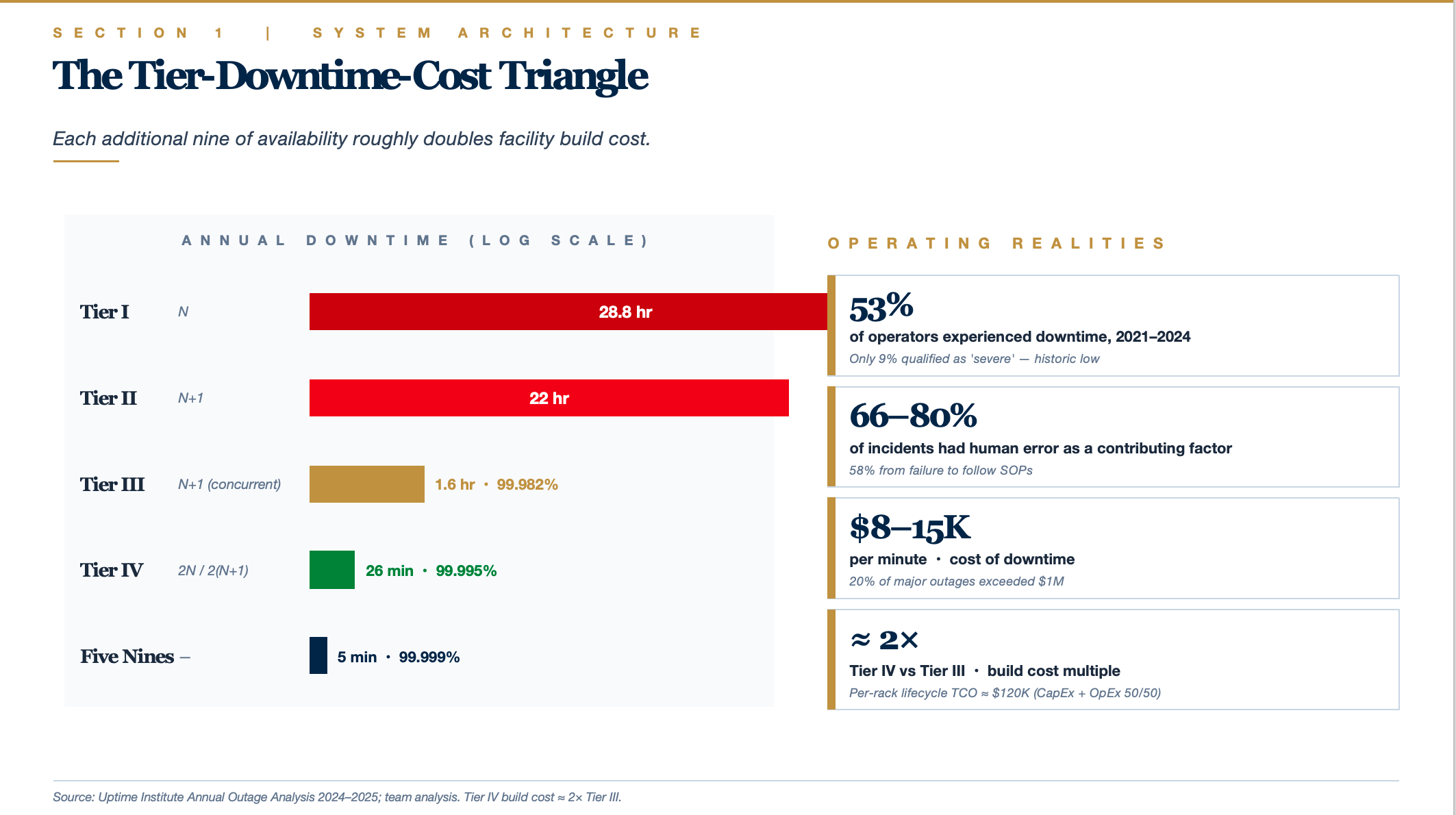
Uptime Institute's 2024–2025 survey reports that 53% of operators experienced downtime between 2021 and 2024, though only 9% qualified as "severe" (a historic low). Human error was a contributing factor in 66–80% of incidents, with 58% attributable to failure to follow standard operating procedures. 54% of respondents reported that their most recent major outage cost exceeded $100K, and roughly 20% exceeded $1M.
Tier IV facilities cost approximately twice as much to build as Tier III. Per-rack lifecycle TCO runs around $120,000 (CapEx and OpEx each accounting for roughly 50%). The core decision calculus: at a downtime cost of $8,000–$15,000 per minute, determine whether the incremental redundancy investment of Tier IV is justified by the avoided outage losses.
Battery Energy Storage Systems (BESS): Lithium-Ion Dominance & Emerging Technologies
0 ms ──── 30 s ──── 5–15 min ──── Hours ──── Days
   UPS interval         Legacy UPS limit       Genset interval
Traditional VRLA batteries cannot perform the genset's job because of two hard constraints:
- Low energy density: 35–40 Wh/kg — storing hours of energy would require a battery room larger than the data hall itself.
- Short cycle life: 500–1,200 cycles — daily charge/discharge for peak-shaving would exhaust the batteries within 2 years.
LFP lithium-ion technology shatters both constraints:
- Energy density 4–5× greater (140–190 Wh/kg)
- Cycle life 5–10× longer (3,000–5,000+ cycles)
- Price collapse ($108/kWh — already below the full-lifecycle cost of a diesel-genset system)
The implication: for the same footprint, stored energy jumps from "5 minutes" to "80 minutes or even several hours" — landing squarely in the time window that diesel gensets previously monopolized.
The New Three-Tier Functional Allocation
| Time Horizon | Legacy Solution | Lithium-Ion BESS Solution |
|---|---|---|
| 0–30 s | UPS (VRLA) | BESS |
| 30 s – 80 min | Diesel genset | BESS (same system continues to supply load) |
| 80 min – Days | Diesel genset | Diesel genset / gas turbine / utility restoration |
Microsoft's Stackbo deployment — a 16 MWh / 24 MW system — embodies this logic: 80 minutes at full load means:
- Sub-50 ms response (replacing the UPS)
- Full-load sustain for 80 minutes (covering the genset's near-term role)
- Utility restoration probability within 80 minutes is > 95% (Nordic grid statistics), drastically reducing genset dispatch frequency
BESS can respond within 50 milliseconds of an outage — more than sufficient to bridge the 10–30 second gap before generators start. More consequentially, BESS is evolving toward diesel-genset displacement: Microsoft deployed 16 MWh of BESS (24 MW peak) at Stackbo, Sweden, delivering 80 minutes of full-load backup; Google installed 2.75 MW / 5.5 MWh batteries at St. Ghislain, Belgium, as a diesel-genset replacement; and as of 2025, Google has deployed more than 100 million lithium battery cells (hundreds of MWh) across its global data center fleet.
BESS as an Active Revenue Generator — The Truly Disruptive Element
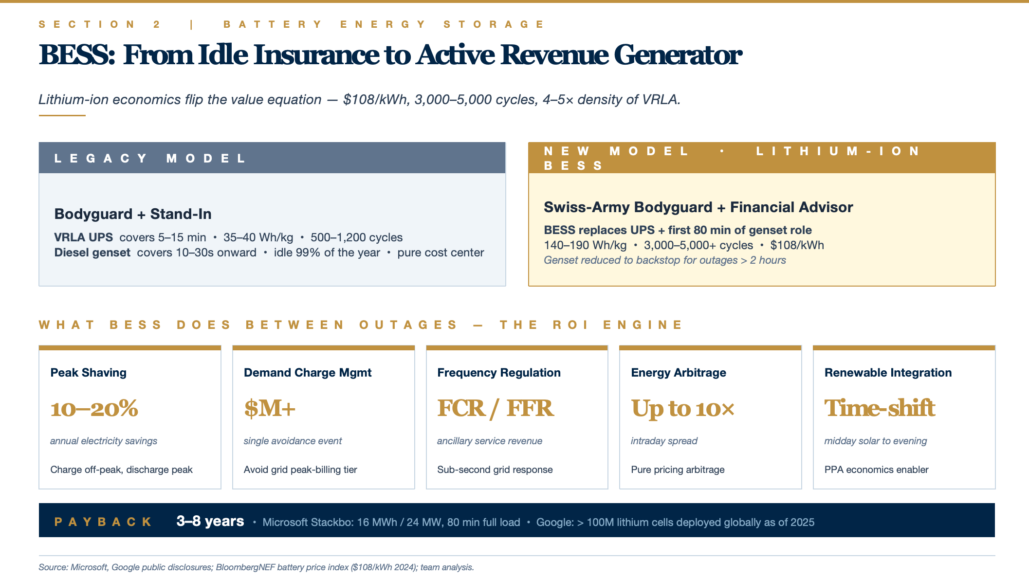
A diesel genset sits idle 99% of the year, runs a monthly test cycle, and is a pure cost center. Lithium-ion BESS works for its keep between outages — this is why the ROI comes in at 3–8 years. It is not "buying insurance" but rather "buying insurance that moonlights as a profit center." Diesel has no equivalent attribute.
- Peak shaving / valley filling: Charge during off-peak tariff windows, discharge during peak hours — saving 10–20% on annual electricity costs.
- Demand-charge management: Avoid triggering the grid's peak-demand billing tier — a single avoidance event can save millions of dollars.
- Grid frequency regulation (FCR / FFR): Participate in ancillary-service markets, earning revenue by responding to grid frequency deviations within seconds.
- Energy arbitrage: Intraday electricity price differentials reach up to 10× — pure arbitrage income.
- Renewable integration: Store excess midday solar generation for evening dispatch.
The more precise framing, therefore, is not "lithium batteries serve as both UPS and genset" but rather: lithium-ion BESS absorbs 100% of the UPS function + the genset's short-to-medium-duration (< 2 hour) backup function + adds an entirely new energy-management revenue stream. The diesel genset is compressed to a backstop role for long-duration outages (> 2 hours) only.
Analogy:
- Legacy model: Bodyguard (UPS) + long-term stand-in (diesel genset)
- New model: Swiss-army-knife bodyguard (BESS — also moonlights as a financial advisor between incidents) + emergency reserve (diesel / gas, deployed only in extreme scenarios)
The Most Aggressive Architectures — Two Emerging Scenarios
1. AI Training Clusters (Microsoft Fairwater et al.)
- UPS eliminated entirely (training workloads can checkpoint and resume)
- Minimal BESS retained for sub-second protection
- Diesel or gas turbine provides long-duration backstop
- Overall backup-power investment drops substantially
2. Self-Powered Hyperscale Campuses (xAI Memphis)
- On-site combined-cycle gas power plant (grid-independent)
- BESS handles frequency regulation and short-duration backup
- Diesel gensets replaced by gas turbines
- Essentially: "the campus becomes its own utility"
GPU Compute Hardware Is Rewriting Power Density Rules
Average data center rack power density evolved from ~4 kW in 2011 to ~12 kW by 2024 (AFCOM data), but AI accelerators are pushing high-end requirements into an entirely different order of magnitude. NVIDIA GPU power draw is scaling aggressively across generations: A100 (400 W) → H100 (700 W) → B200 (1,000–1,200 W) → GB200 Superchip (2,700 W for 2 GPUs + 1 Grace CPU).
NVIDIA GB200 NVL72 is the current benchmark for high-density systems: a single rack integrates 72 Blackwell GPUs + 36 Grace CPUs with 13.5 TB HBM3e memory, delivering 1.44 exaFLOPS (sparse FP4), consuming 120–140 kW per rack, and weighing 1.36 metric tons. Coolant enters at 2 L/s (25 °C) and exits with a ≈ 20 °C temperature rise. GPUs and CPUs are liquid-cooled; NICs and storage are still air-cooled by 40 mm fans. NVIDIA's next-generation Vera Rubin NVL144 (2026) is projected to push per-rack power to ~600 kW.
The Fundamental Equation Behind Every Distribution Challenge
All data center power-distribution challenges reduce to one identity: P = U × I
- P = Power (watts)
- U = Voltage (volts)
- I = Current (amps)
At a given power level, lower voltage means higher current. And high current introduces three compounding problems:
Problem 1: Conductor cross-section becomes physically untenable
Higher current demands thicker copper; cost and weight scale non-linearly. At 48 V, the GB200 NVL72 requires 3,800 amps — copper busbars of that rating physically cannot fit inside a standard rack.
| Current | Typical Conductor | Unit Weight | Diameter |
|---|---|---|---|
| 30 A | Residential wiring | Light | A few mm |
| 350 A | 500 MCM cable | Several kg/m | Thumb-thick |
| 3,800 A | Massive copper busbar | Tens of kg/m | Brick-sized |
Problem 2: I²R losses scale with the square of current
Resistive heating = I² × R. Double the current and losses quadruple. At 3,800 A flowing through any busbar segment, the heat generated would be sufficient to cook the rack.
Problem 3: Voltage drop (IR drop) spirals out of control
Higher current over longer runs produces severe voltage sag. At 3,800 A flowing through 1 meter of busbar, the drop can reach several volts — on a 12 V bus, this means the chip receives unstable voltage, directly impairing computational reliability.
These three effects combine to form the physical basis for Schneider Electric's widely cited conclusion: "400 V three-phase AC and 48 VDC solutions become strained at 200 kW/rack and are entirely infeasible at 400 kW/rack." This is not a matter of engineering effort — it is a matter of physics.
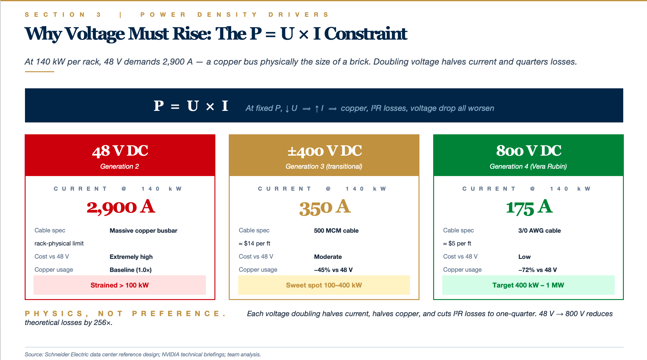
Comparative Impact at 140 kW — Same Power, Different Voltages
| Voltage Architecture | Required Current | Cable Specification | Approx. Unit Cost | Copper Usage |
|---|---|---|---|---|
| 48 VDC | ~2,900 A | Massive copper busbar | Extremely high | Baseline |
| ±400 VDC | ~350 A | 500 MCM cable | $14/ft | −45% |
| 800 VDC | ~175 A | 3/0 AWG cable | $5/ft | Halved again |
Each voltage doubling halves the current, halves the copper, and cuts losses to one-quarter. Going from 48 V to 800 V reduces current by 16× and theoretical losses by 256× — this is the core attraction of high-voltage DC.
In other words, the voltage-architecture upgrade is not "performance optimization" — it is a physical necessity. The evolutionary path: Legacy AC → 48 V → ±400 V → 800 V.
Generation 1: Legacy 480 V AC + 12 V DC (Power Density < 30 kW/rack)
MV AC → 480 V / 415 V AC → UPS → PDU → Server PSU (AC → 12 V DC) → Motherboard
Each server carries its own PSU performing AC-to-12 V DC conversion. This works fine below 30 kW per rack.
Generation 2: 48 V DC Rack-Level Architecture (30–100 kW/rack)
In 2016, Google contributed the specification to OCP (Open Compute Project). The key change: relocating AC-to-DC conversion from individual servers to the rack level.
480 V AC → Rack-level rectifier → 48 V DC bus → Per-server DC-DC step-down to 12 V
Benefits:
- Eliminates redundant conversion losses from dozens of per-server PSUs
- 48 V delivers 30%+ lower distribution losses than 12 V (at the same power, current drops to 1/4 and I²R losses to 1/16)
- 48 V remains classified as Extra-Low Voltage (ELV) (< 60 V) — no specialized electrical licensing required; a low safety-compliance threshold
Open Rack v3 standardized this as the de facto OCP power architecture. But the GB200 immediately pushed this scheme to its limits — a 120 kW rack at 48 V requires busbars rated at 2,900 A minimum, which is already physically marginal.
Generation 3: ±400 V DC (100–400 kW/rack)
±400 V does not mean the voltage oscillates between +400 V and −400 V (that would be AC). Its actual meaning is a three-wire system:
+400 V ────────────┐
                   │
   0 V ────────────┤  ← Neutral / reference conductor (optional)
                   │
−400 V ────────────┘
- One positive bus (+400 V) at 400 V above ground
- One neutral conductor (0 V) serving as reference
- One negative bus (−400 V) at 400 V below ground
Transitional Advantage 1: 800 V Working Voltage, but Only 400 V to Ground
Electrical safety standards are based on voltage-to-ground, not line-to-line voltage. A ±400 V system delivers:
- Equipment working voltage: 800 V (line-to-line) → enjoys the full benefit of high-voltage / low-current operation (copper halved)
- Voltage-to-ground: only 400 V (each conductor to ground) → insulation requirements, protection design, and safety thresholds equivalent to a 400 V system
Insulation costs and current-related safety expenses are substantially lower than a unipolar 800 V system.
Transitional Advantage 2: Multi-Voltage Supply from a Single Bus
- High-power loads (GPU compute units): tap across +400 V and −400 V for the full 800 V
- Medium-power loads (fans, control boards): tap +400 V to 0 V, or 0 V to −400 V, for 400 V half-bus
A single distribution system delivers two voltage tiers simultaneously — greatly increasing flexibility.
Transitional Advantage 3: Fault Tolerance
If the +400 V bus faults, the −400 V side can continue to operate independently (at reduced power). A unipolar 800 V system loses everything when a single conductor fails.
Transitional Advantage 4: Neutral-Current Cancellation
When the positive and negative loads are balanced, the currents on the two buses are equal and opposite, so the net neutral-wire current approaches zero. This allows the neutral conductor to be significantly thinner than the main buses — or, in some configurations, eliminated entirely — saving additional copper.
NVIDIA's published data: 45% reduction in copper usage relative to a 48 V architecture at equivalent power levels.
Challenges
- Enters the Low Voltage (LV) regulatory domain (> 60 V), requiring licensed electricians and more stringent insulation, clearance, and isolation design.
- DC arc extinguishment is inherently harder than AC (AC naturally crosses zero 100 times per second, extinguishing arcs automatically; DC arcs burn continuously) — dedicated DC circuit breakers are required.
- Electrical-shock risk increases materially, necessitating redesigned grounding and protection schemes.
Generation 4: 800 V DC (400 kW – 1 MW/rack)
NVIDIA's Vera Rubin platform moves directly to 800 V DC — this is the architecture prepared for the 2026–2027 GPU generation. At 800 V, 140 kW requires only 175 A, served by a single 3/0 AWG cable (roughly the diameter of kitchen-appliance wiring).
Why the jump from ±400 V to 800 V? Because post-Rubin generations (Feynman?) may push per-rack power directly to 600 kW – 1 MW, at which point even ±400 V becomes insufficient.
Where does 800 V DC come from? The electric vehicle industry. Tesla, Porsche Taycan, and Hyundai's E-GMP platform all adopted 800 V architectures to reduce charging times and copper mass. AI data centers are essentially borrowing a decade of EV electrical-engineering maturity — the same physics (high power, constrained space, copper cost) yields the same solution.
A Key Architectural Shift — The Integrated Power Shelf
Legacy server racks: Each 1U server carries 1–2 PSUs; a single rack may contain 80 PSUs, each independently performing AC-to-DC conversion.
GB200 NVL72 architecture:
- The entire rack is powered by a small number of centralized power shelves performing AC-to-DC conversion
- Rack-level BBU (Battery Backup Unit): Lithium-ion modules installed directly within the rack or at the end of the rack row
- Converted DC is distributed via a busbar — a thick copper bar running the length of the rack — to all compute and switch trays
- Individual compute nodes no longer carry their own PSUs; they draw power directly from the busbar
Benefits:
- Higher conversion efficiency (large power supplies outperform small ones)
- Simplified maintenance (power shelves are hot-swappable; a single-shelf failure does not affect others)
- Recovered rack space (PSUs are no longer distributed across every server)
- Combined with DC distribution, whole-rack efficiency improves from ~85% to ~95%+
Investment Map Across the Electrical Architecture Stack
L2 Facility-Level Electrical Systems → Traditional Electrical-Equipment Majors' Home Turf
- Schneider, Vertiv, Eaton, ABB, Huawei Digital Power
- Barriers to entry: engineering capability, safety certifications, global service networks
- Business model: project-based + recurring service fees
L3 Rack-Level Energy Storage (L2 Function Pushed Down to L3) → Rack BBU
The core catalyst is NVIDIA's designation of rack BBU as standard equipment on GB200 / GB300 NVL72, and the power-density step-up creating a standalone market for in-rack energy-storage modules.
Li-ion cell → BBU module → BBU system integration → Rack OEM integration → End customer
  (Cell)       (Pack + BMS)  (incl. PCS, controls)   (ODM / server vendor)   (Hyperscaler)
The greatest beneficiaries in this chain are upstream cell manufacturers and power / BBU system integrators, because:
- Per-rack BBU value is $20K–$50K — a 5–10× uplift over traditional UPS per-rack value
- Penetration is starting from near-zero (GB200 has only just entered volume production); the next 3–5 years represent the penetration-rate inflection
- The technology moat lies in "high density + high safety + liquid-cooling compatibility," not commodity cell competition
L1 Self-Build Power Generation → Energy Companies' Home Turf
The core catalyst is North American grid-interconnection queues of 5–7 years and AI training campuses' demand for 100–500 MW-class power, forcing the emergence of "build your own power plant" models.
Gas turbine / reciprocating engine → BOP auxiliaries → EPC → Gas supply → Data center operator
     (Core prime mover)               (Support systems)  (Constructor)  (Upstream energy)
Gas turbines (scarcest — order books are booked out through 2028+):
- GE Vernova (GEV): Global gas-turbine leader; exceptional order visibility; primary supplier for xAI Memphis, Meta, and other AI campuses
- Siemens Energy (ENR.DE): European counterpart; equally saturated order book
- Mitsubishi Heavy Industries (7011.T): Japanese competitor; H-class large-frame turbines are credible contenders
The Convergence: Two Emerging Verticals Funneling into the Same Company Profiles
Both the "L2 function push-down to L3" and the "L1 self-build push-up" trends ultimately converge on the same class of companies: Vertiv (VRT), Schneider Electric (SU.PA), Eaton (ETN), ABB (ABBN.SW).
These four are the full-stack integrators of data center mechanical-electrical systems:
- L2 legacy business (UPS, switchgear, cooling) → stable cash-flow engine
- L3 push-down business (rack BBU, CDU, busbar) → growth engine
- L1 push-up business (microgrid integration, MV distribution) → new revenue vector
Vertiv (VRT) is the purest embodiment of this thesis over the past three years — spanning liquid cooling to BBU to MV distribution — the quintessential "picks-and-shovels" play for AI data center M&E.
Investment Lens on the Power Density Evolution
Three Generations Side by Side
| Architecture | Era | Per-Rack Power | Role |
|---|---|---|---|
| 48 V DC | 2016–2024 | < 100 kW | Previous-generation mainstream |
| ±400 V DC | 2025–2027 | 100–400 kW | Transitional |
| 800 V DC | 2027+ | 400 kW – 1 MW | Next-generation target |
±400 V sits in the middle — it is neither the technological endpoint (unipolar 800 V is cleaner) nor a greenfield architecture (it leverages a large body of mature low-voltage AC engineering). This posture — "one step forward but not quite all the way across" — is the hallmark of a transitional technology.
If the supply chain were ready, theory would dictate going straight to unipolar 800 V — simpler, more copper-efficient, and more headroom for future scaling. In practice, that leap is not yet possible, for reasons distributed across four layers.
Layer 1: Generational Thresholds in Electrical Safety Standards
Voltage is not a continuous variable in engineering standards — it operates as a stepped classification:
| Category | Range | Regulatory Implications |
|---|---|---|
| Extra-Low Voltage (ELV) | < 60 V DC | Virtually no safety constraints; accessible by untrained personnel |
| Low Voltage (LV) | 60 V – 1,500 V DC | Requires licensed electricians, insulation-class requirements, mandatory grounding protection |
| High Voltage (HV) | > 1,500 V DC | Entirely separate engineering codes and dedicated equipment |
48 V falls within the ELV regime; 800 V falls within the LV regime — between these two domains lies a full chasm of regulation, training, and construction codes.
A direct jump from 48 V to 800 V would require:
- Industry-wide electrician retraining
- A complete rewrite of insulation, clearance, and grounding standards
- Updates to IEC, UL, GB, and other safety-certification frameworks
- Reassessment of risk pricing by insurance underwriters
None of this can be accomplished in one or two years. ±400 V sits in the lower portion of the LV domain, allowing the industry to acclimate to the "LV DC" paradigm while safety standards mature incrementally.
Layer 2: DC Circuit-Breaker Maturity
This is the hardest engineering bottleneck.
AC arc extinguishment comes "free"; DC arc extinguishment is fundamentally difficult. AC current passes through zero 100 times per second (at 50 Hz), so a breaker merely needs to open at the zero crossing and the arc self-extinguishes. DC has no zero crossing — once an arc strikes, it burns continuously until its energy is dissipated. Higher voltage means higher arc energy and harder extinguishment.
DC circuit-breaker maturity stratified by voltage:
| Voltage Level | DC Breaker Maturity | Commercialization Status |
|---|---|---|
| 48 V DC | Fully mature | A few dollars each; ubiquitous |
| 400 V DC | Mature (borrowed from solar PV and EV) | In commercial use 5+ years |
| 800 V DC | Recently commercialized | Sourced from latest EV platforms; expensive, limited selection |
| 1,500 V DC | Solar-PV domain only | No rack-level products exist |
The advantage of ±400 V: each bus conductor is 400 V to ground, so the system can use existing, proven 400 V DC breakers — devices that have been validated at scale in the solar-PV industry (string voltages typically 600–1,000 V, module-level voltages 400–500 V) and the EV industry (800 V platforms are in fact ±400 V architectures). Pricing is already competitive.
A direct move to unipolar 800 V would require breakers rated for 800 V to ground — devices that are currently scarce, expensive, and unproven in large-scale data center environments.
Layer 3: Voltage Withstand of Server-Side Power Semiconductors
This layer is often overlooked in analysis. The power shelf in the rack and the DC-DC converters inside the server ultimately need to step the high-voltage DC bus down to < 1 V for the die. The critical devices in this step-down chain are power semiconductors (MOSFETs, SiC, GaN), each with a rated voltage ceiling.
| Device | Mainstream Voltage Rating | Data Center Application |
|---|---|---|
| Silicon MOSFET | 100 V – 600 V | Workhorse for 48 V / 400 V systems |
| SiC MOSFET | 650 V / 1,200 V / 1,700 V | Core device for 400 V / 800 V systems |
| GaN HEMT | 100 V – 650 V | High-frequency applications; complements SiC |
1,200 V SiC power devices have only reached true volume production with acceptable pricing in the past two years. For a ±400 V power shelf, a 1,200 V SiC is sufficient (800 V line-to-line + safety margin ≈ 1,200 V).
A unipolar 800 V system, however, presents 800 V to ground; transient voltages at certain internal nodes can spike to 1,500 V+, necessitating 1,700 V or even 2,000 V SiC — devices that only began shipping in volume in 2025, with yields and costs still unfavorable.
Deploying ±400 V first to build market volume, then allowing 1,700 V SiC a 2–3 year maturation window — this is the industry's actual cadence.
Layer 4: Electrician Skill Sets & Construction Codes
This layer is "soft" but critical. The global data center construction workforce has spent the past 30 years on low-voltage AC distribution (380 V / 480 V); 48 V DC is manageable because of its low voltage. Suddenly asking these teams to install 800 V DC systems means:
- AC conductor-sizing rules no longer apply
- Grounding systems must be redesigned (IT / TT / TN grounding schemes have different implications under DC)
- Maintenance safety procedures change fundamentally (DC cannot rely on "wait for zero crossing before opening")
- Fault-diagnostic instruments and methodologies must be replaced entirely
±400 V, in many construction details, borrows from 480 V three-phase AC conventions (conductor gauge, grounding topology, and insulation class are nearly aligned), making the learning curve for construction crews significantly gentler. This is an advantage that unipolar 800 V does not share.
The Strategic Conclusion
±400 V is a near-perfect compromise — capable of supporting the current GB200 / GB300 generation (120–200 kW/rack) while also handling the next GPU generation (300–400 kW/rack), extending infrastructure useful life to 5–7 years. By the time per-rack power pushes past 600 kW in 2027–2028, 800 V standards, SiC devices, and construction codes will all have matured — making the 800 V transition a natural progression.
But if ±400 V Is Merely Transitional — Investment Implications
- ±400 V-specific equipment, chips, and cabling will enjoy a 3–5 year sweet spot, but the ceiling is capped — capacity and pricing will be compressed by the post-2027 wave of 800 V adoption.
- The true long-term beneficiaries are "voltage-agnostic" suppliers — companies whose power shelves, busbars, breakers, and SiC devices work across both 400 V and 800 V, harvesting the transitional dividend and seamlessly pivoting into the 800 V era.
- Pure 48 V players will be rapidly displaced: If a company's core product for the past decade has been 48 V power shelves, it has roughly 2 years to pivot or face marginalization.
The Most Telling Signal Points
- NVIDIA's own roadmap is the clearest tell: GB200 ships with ±400 V; Vera Rubin moves directly to 800 V — an explicit signal to the supply chain that the transitional window is roughly 2 years.
- Schneider, Vertiv, and Delta Electronics are all developing dual product lines (±400 V and 800 V simultaneously), not betting on the transitional architecture itself.
- SiC leaders (Wolfspeed, Infineon, ROHM) are concentrating capital investment on 1,700 V capacity rather than 1,200 V — they are positioning for the 800 V era.
Network Interconnects & Modular Architecture Trends
Spine-Leaf Architecture as the De Facto Standard
1. North-South vs. East-West Traffic
North-South traffic: Traffic flowing between external users and the data center. For example, a user opening a web application — the request travels from the phone into the data center, locates the server, and returns the page. This is north-south.
East-West traffic: Traffic flowing among servers within the data center. For example, a web application server querying a database, calling a recommendation service, and reading a Redis cache — all of these exchanges occur entirely inside the data center.
The evolution of traffic ratios:
| Era | North-South | East-West | Dominant Workload |
|---|---|---|---|
| 2000s | ~80% | ~20% | Monolithic applications, static web pages |
| 2010s | ~50% | ~50% | Virtualization, early microservices |
| Modern (2020s) | < 30% | > 70% | Microservices, distributed databases |
| AI training clusters | < 5% | > 95% | Inter-GPU gradient synchronization |
Why the dramatic shift? Because application architecture moved from monolithic to distributed. A single user request may traverse 50 microservices, query 10 databases, and hit a cache 100 times — all east-west traffic.
In AI training the ratio becomes even more extreme — training a model like GPT-4 generates 95%+ network traffic as inter-GPU gradient-synchronization communication, with near-zero north-south traffic.
This shift single-handedly killed the traditional three-tier architecture — a topology purpose-built to optimize north-south flows.
2. Why the Traditional Three-Tier Architecture Failed
The legacy data center network was a tree-structured Core → Aggregation → Access hierarchy:
           ┌──────────┐
           │   Core   │  ← Core layer (2–4 very large switches at the apex)
           └────┬─────┘
                │
        ┌───────┴────────┐
        │                │
   ┌────┴────┐      ┌────┴────┐
   │ Aggreg  │      │ Aggreg  │  ← Aggregation layer
   └────┬────┘      └────┬────┘
        │                │
    ┌───┴───┐        ┌───┴───┐
    │Access │        │Access │  ← Access layer (server-facing)
    └───────┘        └───────┘
This architecture has three fatal shortcomings:
Problem 1: East-west traffic is forced to "take the long way around"
Server A attached to the left access switch wants to reach Server B on the right — traffic must climb all the way to the core and back down to the opposite access switch, traversing 4–6 hops minimum. Each hop adds several microseconds of latency.
Problem 2: Severe bandwidth oversubscription
An access switch may have 48 × 10G = 480 Gbps of downlink capacity, but only 4 × 10G = 40 Gbps of uplink — a 12:1 oversubscription ratio. This was acceptable when north-south traffic dominated (user requests never saturated 480G simultaneously), but east-west bursts instantly congest the uplinks.
Problem 3: STP blocks half the links
To prevent loops, the legacy architecture ran STP (Spanning Tree Protocol), which proactively blocks redundant links, leaving only a single active path. The result: you paid for 8 uplinks, but only 4 are operational — the other 4 "sleep" until a primary link fails.
Bandwidth utilization is abysmal.
3. How Spine-Leaf Solves It: The Elegance of the Clos Network
Charles Clos designed a multi-stage non-blocking topology for telephone switching networks in 1952 — rediscovered by data centers 70 years later. The core idea: use only two tiers, but connect every Leaf to every Spine.
Spine tier:   [S1]    [S2]    [S3]    [S4]
               │╲╲╲╲  ╱╱╱╱╲╲╲╲  ╱╱╱╱│
               │ ╲╲╲╲╱╱╱╱  ╲╲╲╲╱╱╱╱ │
               │  ╱╱╱╱╲╲╲╲  ╱╱╱╱╲╲╲╲│
               │ ╱╱╱╱╲╲╲╲  ╱╱╱╱╲╲╲╲ │
Leaf tier:    [L1]    [L2]    [L3]    [L4]
               │       │       │       │
             Servers  Servers Servers Servers
Key structural properties:
- Every Leaf connects to every Spine — forming a complete bipartite graph
- Servers connect only to Leaves; Spines do not interconnect
- Leaves do not interconnect with each other
This structure produces three fundamental improvements:
Improvement 1: Any two servers are at most 2 switch hops apart
Server A → Leaf1 → Spine2 → Leaf3 → Server B. Always 2 switch hops, yielding predictable, stable latency.
Improvement 2: ECMP puts all links to work simultaneously
ECMP (Equal-Cost Multi-Path): Leaf1 has 4 uplinks to 4 Spines? The routing protocol (BGP / OSPF) hash-distributes traffic across all 4, with every link operating at capacity. No STP "sleeping links."
Bandwidth utilization jumps from ~50% to ~95%+.
Improvement 3: Horizontal scale-out
Need more bandwidth? Add Spines. Need more ports? Add Leaves. Two dimensions scale independently. Unlike the three-tier model, where the core layer hitting its limit forced a full-architecture teardown and rebuild.
4. What Is the Scale Ceiling?
Two-tier Clos (standard Spine-Leaf) — Theoretical limit:
Assume 64-port 800G switches as Spines, 32 ports facing Leaves and 32 reserved for redundancy:
- Spine count = 32 (every Leaf connects to every Spine)
- Leaf count = 64 (every Spine connects to every Leaf)
- Each Leaf serves 32 downstream servers
- Total: 32 × 64 = 2,048 Leaf-facing ports → approximately 6,000 servers (accounting for practical oversubscription and headroom)
Five-stage Clos (also called three-tier Clos / Super-Spine architecture):
When two tiers are insufficient, a third "Super-Spine" tier is added, interconnecting multiple Spine-Leaf modules (called Pods):
              Super-Spine (top tier)
             ╱      │      │      ╲
        Spine-A  Spine-B  Spine-C  Spine-D
           │       │       │       │
         Leaves  Leaves  Leaves  Leaves
           │       │       │       │
        Servers Servers Servers Servers
        (Pod 1)  (Pod 2)  (Pod 3)  (Pod 4)
Why "five stages"? Because from source to destination a packet traverses 5 switching elements: Leaf → Spine → Super-Spine → Spine → Leaf.
This architecture supports 100,000+ hosts — the scale at which Meta, Google, and xAI operate their largest clusters. In AI training clusters, each Pod typically corresponds to a "GPU training compartment" (e.g., 1,024 GPUs), with inter-Pod communication traversing the Super-Spine.
5. The Routing Protocol Stack: eBGP + EVPN + VXLAN
Why three protocols? Because a modern data center network must solve three distinct problems.
Problem A: How do switches discover each other? → eBGP (Underlay)
Underlay = the physical network layer. Leaves and Spines need a routing protocol to exchange "where I am and what I can reach" information.
Historically OSPF was common, but modern data centers overwhelmingly choose eBGP (External BGP), for these reasons:
- BGP was designed as the Internet backbone protocol — it natively supports massive scale
- Configuration assigns each switch its own AS (Autonomous System) number, delivering excellent fault isolation
- Unifies with WAN routing protocols, producing a consistent operations model
- Native, mature ECMP support
This is the basis for the statement that "eBGP is the dominant Underlay protocol."
Problem B: How do VMs / containers communicate across subnets? → VXLAN (Overlay)
Overlay = a logical network layered on top of the physical network.
A modern physical server runs dozens of VMs or containers, potentially belonging to different tenants and subnets. VXLAN (Virtual Extensible LAN) encapsulates Ethernet frames inside UDP packets, allowing VMs to behave as if they share a single VLAN while the underlying physical network can be any topology.
Analogy: VXLAN is like a shipping container — it packages diverse parcels (VM traffic) into standardized containers (VXLAN packets) for transport across the physical network, then unpacks them at the destination.
Problem C: Which VM is on which server? → EVPN (Control Plane)
VXLAN solves "how to encapsulate" but not "where to send." EVPN (Ethernet VPN) is VXLAN's "address book" — each Leaf uses EVPN to announce to all other Leaves: "I have VM-A and VM-B attached; their MAC/IP addresses are xxx."
How the three work together:
Application:   VMs / Containers
                ↕ (transparent)
Overlay:       VXLAN (data encapsulation) + EVPN (control signaling)
                ↕ (runs on top of the physical network)
Underlay:      eBGP (physical routing)
                ↕
Physical:      Spine-Leaf switches + fiber optic cabling
This stack has been the "standard answer" for data center networking over the past decade — the underlying network architecture of AWS, Azure, and Alibaba Cloud all follows this paradigm.
6. The Data Center Switching ASIC Landscape: Broadcom Dominance and the Breakout Attempts
Broadcom Tomahawk 5: The Reigning Champion
Broadcom Tomahawk 5 (51.2 Tbps, 64 × 800 GbE) — released in 2023 — is the flagship switching ASIC and the de facto standard for 800G-class data center switches.
- 51.2 Tbps: Single-chip aggregate switching capacity
- 64 × 800 GbE: 64 ports of 800G Ethernet
- Commands 60%+ share of the merchant data center switching-ASIC market
The next-generation Tomahawk 6 has been announced with bandwidth doubling to 102.4 Tbps — 2026 marks the inaugural year for 1.6T-port switching.
Three Vendor Strategies
Strategy A: Buy Broadcom silicon, build the box
- Arista (ANET): Uses Tomahawk 5; differentiates through its EOS operating-system software. The "Arista 7060X6 series" exemplifies this path. Holds 18.9% of the data center switching market — second only to Cisco.
- White-box switch ecosystem: ODMs such as Edgecore, Celestica, and Quanta sell bare Broadcom-powered hardware; customers install their own network OS (SONiC, Cumulus). Microsoft, Meta, and Google are major white-box buyers.
Strategy B: In-house ASIC development
- Cisco Silicon One G300: Cisco's proprietary ASIC powering high-end Nexus 9000 models. Recognizing the strategic risk of Broadcom dependency, Cisco has invested billions over the past five years in custom silicon.
- NVIDIA Spectrum-X: Born from the Mellanox acquisition — an AI-network-optimized ASIC pursuing both InfiniBand and Ethernet markets.
- Marvell Teralynx 10: Broadcom's largest merchant-silicon competitor; adopted by AWS and other hyperscalers.
Strategy C: Hyperscaler captive ASICs
- Google: Proprietary Aquila networking silicon
- Amazon: Proprietary network ASIC (SiCortex lineage)
- Meta: Internal white-box program
The high-end data center switching-ASIC market is dominated by a single player — Broadcom — and everyone else is attempting to break out.
400G / 800G Optical Interconnects Entering Large-Scale Deployment
AI Data Center Optical Interconnect Market
                    (2024: $9B → sustained high growth)
                                │
              ┌────────────────┴──────────────────┐
              │                                    │
        Product Generation                   Technology Route
              │                                    │
      ┌───────┼────────┬───────┐        ┌──────┼──────┐
     100G   400G    800G    1.6T       SiPh    CPO    LPO
                                       50%    Hyper-  Transi-
                                      share   scaler  tional
                                      2027    first   solution
                                              choice  2024+
                                              2026+
Short-distance data transport has two paths: copper and fiber.
The physics of copper transmission:
- Signals propagate as electromagnetic waves in copper; attenuation rises steeply with speed
- At 100 Gbps on copper, the effective reach is only 3–5 meters
- At 200 Gbps this shortens to 1–2 meters
- At 400 Gbps copper is essentially unusable — unless DAC (Direct Attach Copper) is employed at extremely short distances
The physics of fiber:
- Signals are light pulses propagating through glass fiber at near-light speed
- Attenuation is minimal — single-mode fiber can run 10 km with very low loss
- Bandwidth is virtually unlimited (theoretically reaching multi-Tbps)
Data center reality:
- Intra-rack (< 2 m): copper / DAC (cheapest)
- Inter-rack (within a row, meters to tens of meters): fiber is mandatory (multimode fiber + optical transceiver)
- Inter-Pod / inter-hall (tens to hundreds of meters): fiber is mandatory (single-mode fiber)
In AI clusters, GPUs must communicate across racks — a single NVL72 holds only 72 GPUs, but training a GPT-4-class model requires 10,000+ GPUs. This means massive inter-rack communication, all carried over fiber.
What an Optical Transceiver Does
An optical transceiver (optical module) performs one conceptually simple but engineering-extreme task — converting electrical signals into optical signals for transmission, and converting incoming optical signals back to electrical signals.
Physical structure:
Switch ASIC ──electrical──→ [Optical Transceiver]
                             ├── Modulator (E→O) ── fiber ──→
                             └── Detector  (O→E) ←── fiber ←──
                           ──electrical──→ Switch ASIC
Each transceiver plugs into a port on a switch or GPU NIC, bridging racks via a fiber-optic cable. A 51.2 Tbps switch with 64 × 800G ports requires 64 × 800G optical transceivers.
Transceiver count in a GPU cluster:
For a 100,000-GPU training cluster, under typical architecture:
- Each GPU requires 4–8 outbound connections (NVLink Switch / Scale-out)
- All inter-rack segments use optics
- Total transceiver count: hundreds of thousands to over one million units
At a unit price of $700–$1,500 per 800G transceiver, a single cluster's optics alone represent a several-hundred-million to multi-billion-dollar market. This is why optical transceivers are among the most certain high-growth segments in AI infrastructure.
Generational Progression
| Generation | Mainstream Era | Per-Port Data Rate | Module Power | Approx. Unit Price |
|---|---|---|---|---|
| 100G | 2018–2022 | 100 Gbps | 3.5–5 W | $200–400 |
| 400G | 2023–2025 | 400 Gbps | 8–12 W | $500–1,000 |
| 800G | 2024–2026 | 800 Gbps | 14–20 W | $700–1,500 |
| 1.6T | 2025–2027 | 1,600 Gbps | ~25–30 W | $1,500–3,000 |
| 3.2T | 2027+ | 3,200 Gbps | TBD | TBD |
"400G delivers 4× the bandwidth at 2.5–3× the module cost of 100G" — this is the signature of a generational leap: each new generation typically delivers 4× bandwidth for only 2–3× the cost increase, so cost-per-Gbps declines 30–50%. This is why data centers upgrade rapidly once a new generation matures.
Per-Gbps power consumption falls, but absolute module power keeps rising (5 W → 15 W → 25 W). This creates a new engineering problem — the optical transceivers themselves become major heat sources. A 64-port 800G switch dissipates 64 × 18 W ≈ 1.15 kW in transceiver power alone — more than the switching ASIC itself.
Packaging Formats: OSFP / QSFP-DD / OSFP-XD
An optical transceiver's "physical shell + electrical interface" standard is called its form factor. At the same 800G data rate, different form factors yield different thermal and density characteristics.
QSFP-DD (Quad Small Form-factor Pluggable Double Density)
- The traditional mainstream data center form factor
- Compact form factor, high port density (more modules per switch faceplate)
- Drawback: Limited thermal envelope — at 800G, temperatures can exceed safe thresholds
OSFP (Octal Small Form-factor Pluggable)
- Slightly larger than QSFP-DD, with an integrated metal heat-sink fin
- 15 °C cooler than QSFP-DD — a margin sufficient for reliable 800G long-duration operation
- Therefore the preferred form factor for AI high-density 800G deployments — NVIDIA Quantum / Spectrum platforms use OSFP
OSFP-XD (OSFP eXtended Density)
- The 1.6T evolution of OSFP; each module supports 2 × 800G lanes or 1 × 1.6T lane
- The statement that "92% of hyperscaler contracts" have aligned on OSFP-XD refers to the 1.6T-era form-factor consolidation among leading operators
The form-factor debate in essence: QSFP-DD is smaller but thermally constrained; OSFP is somewhat larger but can reliably sustain 800G / 1.6T. AI clusters prioritize reliability over density — a single transceiver failure breaks an entire GPU communication chain — so OSFP wins.
Technology Routes for Power and Cost Reduction
Route A: Silicon Photonics (SiPh)
Conventional transceivers use indium phosphide (InP) or gallium arsenide (GaAs) lasers — expensive processes with limited wafer-scale capacity.
Silicon Photonics integrates optical devices directly onto a silicon die — fabricating photonic elements using CMOS semiconductor processes.
Advantages:
- Leverages existing large-scale semiconductor fabs (TSMC, Intel can both produce them) — cost decreases and capacity elasticity increase
- High integration density (multi-channel optical paths on a single silicon die)
- Projected to capture 50% of the optical transceiver market by 2027
Key players:
- Intel: Earliest mover in SiPh, though commercialization has lagged expectations in recent years
- Zhongji Innolight (300308.SZ): "Shipping SiPh-based modules at volume starting Q2" — SiPh becomes the core technology path for its 1.6T portfolio
- Coherent / Lumentum: Legacy optical-component giants transitioning to SiPh
- Ayar Labs: CPO-focused SiPh startup with a valuation exceeding $1B
Route B: CPO (Co-Packaged Optics)
The most radical route — soldering the optical engine directly adjacent to the switching ASIC.
Conventional topology (pluggable transceivers):
ASIC ── electrical signal (long distance, high power) ── port ── [Pluggable Transceiver] ── fiber
CPO topology:
ASIC ── optical engine (soldered directly beside the die) ── fiber
The electrical-signal path from ASIC to photonic device shrinks from centimeters to millimeters, drastically reducing electrical attenuation. Power drops from ~15 pJ/bit to ~5 pJ/bit (a 65–73% reduction).
Advantages:
- Major power reduction (saves several hundred watts per 51.2T switch)
- Higher density (eliminating the pluggable cage frees PCB real estate)
- Better signal integrity (short-distance electrical transmission)
Disadvantages:
- Not field-replaceable — if the optical engine fails, the entire switch must be swapped
- Maintenance paradigm changes completely (data center operations teams must be retrained)
- Manufacturing process is extremely complex (heterogeneous opto-electronic integration)
If CPO scales, 30–50% of traditional pluggable transceiver demand could be displaced — transceiver vendors must pivot to CPO optical-engine manufacturing or face marginalization. Both Zhongji Innolight and Eoptolink are racing to secure this segment.
Route C: LPO (Linear Pluggable Optics)
The "dark horse" route that emerged suddenly in 2023–2024.
Conventional transceivers include a DSP (Digital Signal Processor) chip responsible for signal compensation, error correction, and equalization — the DSP accounts for 50% of the transceiver's power consumption.
LPO's approach: Remove the DSP entirely — let the switch ASIC's electrical output run "bare" to the photonic device, relying on the intrinsic linearity of the optical path for transmission.
Result: 800G transceiver power drops from 13 W to < 4 W (a 70% reduction).
Advantages:
- A brute-force power-savings approach — no CPO-style manufacturing revolution required
- Retains pluggability (compatible with existing data center architectures)
- Lower cost (eliminates a DSP die)
Disadvantages:
- Effective only at short distances (< 100 m) — insufficient signal compensation for longer reaches
- Imposes higher signal-quality requirements on the ASIC (DSP's former workload shifts to the ASIC side)
LPO vs. CPO:
| Dimension | LPO | CPO |
|---|---|---|
| Magnitude of change | Small (DSP removal) | Large (packaging overhaul) |
| Power reduction | ~70% | ~65–73% |
| Pluggability | Preserved | Sacrificed |
| Commercialization timeline | 2024–2025, already deployed | 2026+ |
| Best-fit scenario | Intra-data-center | Hyperscale deployments |
LPO is the "transition within the transition" — a low-risk solution filling the 2–3 year window before CPO fully matures.
DCI Optics: Pluggable Coherent Technology Reshaping the Interconnect Landscape
The optical transceivers discussed above operate inside a data center — switch-to-switch, GPU-to-GPU, rack-to-rack (meters to hundreds of meters). DCI (Data Center Interconnect) transceivers operate between data centers — linking facilities separated by kilometers to thousands of kilometers (80–2,000 km).
| Dimension | Intra-DC Transceivers | DCI Transceivers |
|---|---|---|
| Growth driver | AI intra-cluster bandwidth demand | Cross-campus training + cloud interconnect |
| Market size | $9B (2024) | $10.7B (2024) |
| Growth rate | ~25–30% | ~13% overall; high-speed segment 145% |
| Concentration | Moderate (top 5 hold ~60%) | High (top 3 hold 70%+) |
| Chinese market influence | Dominant | Relatively weaker |
| Margin profile | High (gross margin 30–40%) | Moderate (gross margin 25–30%) |
| Primary beneficiaries | Zhongji Innolight, Eoptolink, O-Net | Ciena, Marvell, Cisco |
Why DCI Is Fundamentally Harder
Optical signals attenuate in fiber — much more slowly than in copper, but cumulatively over distance:
| Distance | Attenuation | Required Handling |
|---|---|---|
| 100 m | < 0.5 dB | Direct detection |
| 10 km | ~3 dB | Simple detection |
| 80 km | ~16 dB | Optical amplification required |
| 1,000 km | ~200 dB (direct transmission impossible) | Multi-stage amplification + coherent detection |
DCI's core technical challenge: how to faithfully reconstruct a signal after it has traveled hundreds to thousands of kilometers.
Intra-DC vs. DCI Transceiver Comparison
| Dimension | Intra-DC Transceivers | DCI Transceivers |
|---|---|---|
| Typical distance | 100 m – 2 km | 80 km – 2,000 km |
| Typical data rate | 100G / 400G / 800G / 1.6T | 100G / 400G / 800G / 1.2T |
| Key technology | NRZ / PAM4 direct modulation | Coherent modulation + DSP |
| Modulation scheme | Simple (intensity modulation) | Complex (phase + amplitude + polarization) |
| Price | $500 – 1,500 | $5,000 – 50,000 |
| Power | 5 – 25 W | 15 – 25 W |
| DSP complexity | Simple or none (LPO) | Extremely complex (core value proposition) |
| Typical customer | Data center operator | Cloud provider + telecom carrier |
| Market size 2024 | ~$9B | ~$10.7B |
| Core players | Zhongji Innolight, Eoptolink, Coherent | Ciena, Cisco, Huawei, Acacia |
Key differentiators:
- DCI modules cost 10–50× more — because DSP complexity is on a different order of magnitude
- DCI is telecom-grade technology migrating into the data center — legacy players are Ciena, Nokia, and Huawei — telecom equipment vendors
- The core value in a DCI module resides in the DSP die — the optical-component portion is relatively standardized
IP-over-DWDM: The Architectural Simplification Revolution
Legacy DCI Architecture
Data Center A
  ┌───────────┐         ┌────────────────┐         ┌────────────┐
  │  Router / │ ─gray─→ │  Transponder   │ ─color─→│    DWDM    │ ──→ Fiber ──→
  │  Switch   │  optic   │  Chassis       │  optic  │  equipment │
  └───────────┘         │  (proprietary  │         └────────────┘
                        │   coherent)    │
                        └────────────────┘
   IP / Ethernet layer    Coherent optical layer     Optical transport layer
Three independent equipment layers — each from a different vendor, each with its own management plane, each consuming separate floor space.
IP-over-DWDM Architecture
Data Center A
  ┌─────────────────┐         ┌────────────┐
  │  Router / Switch│ ─color─→│    DWDM    │ ──→ Fiber ──→
  │  (ZR module     │  optic  │  equipment │
  │   plugged in)   │         └────────────┘
  └─────────────────┘
   IP + coherent unified       Optical transport layer
A ZR coherent module plugs directly into the router port — the entire transponder-chassis layer disappears.
ZR is the "pluggable coherent module standard" family defined by OIF (Optical Internetworking Forum). Previously, DCI required purchasing Ciena's (or equivalent) proprietary transponder chassis — a rack-sized appliance housing proprietary coherent technology, physically separate from the switch.
The ZR standard's revolutionary impact:
- Multi-vendor interoperability: The OIF standard allows ZR modules from different vendors to be mixed
- Direct insertion into switch / router ports: No standalone transponder chassis required
The resulting benefits:
- CapEx savings of 28–38%: Eliminating an entire equipment tier
- Space savings of 50%+: The transponder room is no longer needed
- Power reduction of 30–40%: One fewer OEO (optical-electrical-optical) conversion stage
- Unified operations: Router and optical layers managed within a single control system
OLS (Open Line System) — The Next Wave
OLS will make the DWDM optical layer itself an open standard, enabling hyperscalers to mix and match equipment from different vendors:
- Amplifiers from Vendor A
- ROADMs (Reconfigurable Optical Add-Drop Multiplexer) from Vendor B
- ZR modules from Vendor C
- SDN control system from Vendor D
The entire DCI industry is undergoing the same "white-boxing" process that data center switching experienced:
| Phase | Switching Industry | DCI Industry |
|---|---|---|
| 1.0 Black Box | Cisco winner-take-all | Ciena / Huawei turnkey solutions |
| 2.0 Merchant Silicon | Broadcom + multiple ODMs | Multi-vendor ZR modules |
| 3.0 White Box + Open Source | SONiC + white-box switches | OLS + open management |
The moats of legacy DCI giants like Ciena are being rapidly eroded by OIF standardization and the bargaining power of hyperscale buyers — this is the most consequential structural shift in the DCI industry.
Evaluation Framework: Data Center Acquisition Due Diligence
Due diligence follows the L1 → L2 → L3 → L4 sequence:
- L1: Confirm the supply ceiling and scalability of power, land, water, and connectivity
- L2: Assess the age and retrofit headroom of M&E systems (liquid-cooling readiness)
- L3: Evaluate rack / Pod power-density ceiling and network topology
- L4: Assess the generational currency of compute hardware (AI-readiness)
0. Executive Summary
Project Name:
Asset Type: (Wholesale / Retail Colo / Enterprise Conversion / AI Training / Edge)
Location:
Seller:
Deal Structure: (Equity / Asset Acquisition / JV)
Asking Price:
Recommendation: Proceed / Proceed with Conditions / Reprice / Pass
Investment Thesis
- One-line investment rationale:
- One-line kill risk:
- Value-creation pathway: (Capacity expansion / Liquid-cooling upgrade / Tenant optimization / Pricing uplift / Operational efficiency)
- Top 3 questions for the Investment Committee:
1.
2.
3.
Evaluation Methodology
A. Fatal-Flaw Gate
- If any single Fatal Flaw item fails, the default recommendation is Pass.
B. Four Core Scoring Dimensions
- As-Is Quality: 35%
- To-Be Upgrade Value: 30%
- Execution Certainty: 20%
- Demand Fit: 15%
C. Valuation — Standalone Module
Valuation is decoupled from the technical scorecard and assessed independently:
- Does the current bid already price in expansion / liquid-cooling / AI premium?
- How much incremental CapEx is required to unlock future value?
- Does the risk-adjusted IRR hold?
1. Deal Snapshot
1.1 Asset Profile
- Asset name:
- City / Campus:
- Year built / Phasing dates:
- Gross building area:
- White-space area:
- Land area:
- Tenure: Freehold / Leasehold / Hybrid
- Current use: Wholesale / Retail / Enterprise captive / Hybrid
- Target use: Maintain current profile / AI upgrade / Conversion
1.2 Capacity & Delivery
- Contracted utility power (MW):
- Actual deliverable IT capacity (MW):
- Currently utilized IT capacity (MW):
- Remaining available capacity (MW):
- Expansion capacity (MW):
- Current prevailing rack density:
- Maximum supportable rack density:
- Current cooling modality:
- Liquid-cooling readiness (L0–L5):
1.3 Commercial Overview
- Occupancy rate:
- Top-5 tenant revenue concentration:
- Largest single-tenant revenue share:
- Weighted Average Lease term (WAL):
- Average unit price ($/kW/month or RMB/kW/month):
- Contractual escalator:
- Current EBITDA:
- Current EBITDA margin:
2. Fatal-Flaw Screen
If any single item fails, the asset does not advance to the weighted scoring phase — unless the deal is restructured with a price adjustment or binding remediation conditions.
| Gate Item | Core Question | Result | Notes |
|---|---|---|---|
| Power accessibility | Is there verifiable, deliverable current / incremental MW — not merely paper MW? | Pass / Fail | |
| Cooling upgrade feasibility | Can the target density be achieved within reasonable CapEx and construction timeline? | Pass / Fail | |
| Structural capacity | Do floor loading, clear height, routing, and live loads support the target AI deployment? | Pass / Fail | |
| Regulatory & permit closure | Are there material obstacles in land-use, EIA, energy review, fire code, grid interconnection, or data compliance? | Pass / Fail | |
| Baseline reliability | Is there a history of major outages, maintenance backlog, or single points of failure? | Pass / Fail | |
| Network minimum threshold | Does the asset meet the carrier / fiber / cloud on-ramp floor required by target tenants? | Pass / Fail |
Fatal-Flaw Conclusion
- Pass: Proceed to full due diligence
- Conditional Pass: Enumerate pre-conditions
- Fail: Recommend Pass / Material reprice
3. As-Is Quality Score (Today Value)
This section answers one question: Is this asset worth acquiring in its current state?
Total: 100 points — used solely to characterize current-state quality; does not substitute for the investment recommendation.
3.1 Power Systems (20 pts)
- Actual deliverable IT MW
- Redundancy architecture (N / N+1 / 2N)
- UPS / genset / switchgear age
- Distribution topology and bottlenecks
- Power quality / harmonics / load balancing
- Electricity tariff terms / PPA / pass-through mechanism
3.2 Cooling & Energy Efficiency (15 pts)
- Current PUE / WUE
- Current cooling architecture
- Current supportable density
- Liquid-cooling readiness
- Redundancy and maintainability
- Verified historical efficiency curves
3.3 Network & Interconnection (15 pts)
- Number of carriers
- Carrier neutrality
- Fiber-path diversity
- MMR capacity
- IX / cloud on-ramp presence
- Latency and cross-network quality
3.4 Physical & Structural (10 pts)
- Construction vintage and major-refresh history
- Floor-loading capacity
- Clear height / column grid / routing pathways
- Flood / seismic / fire / physical security resilience
- Brownfield conversion friendliness
3.5 Operations & Reliability (15 pts)
- Tier / ISO / SOC certifications
- DCIM / BMS / SCADA maturity
- AIOps / predictive-maintenance capabilities
- Historical outage / near-miss record
- Maintenance backlog
- MTBF / MTTR
- Staff-per-MW ratio
3.6 Commercial Quality (15 pts)
- Tenant concentration
- WAL
- Rental levels
- Occupancy rate
- Churn risk
- Renewal probability
- Contract-terms quality
3.7 Compliance & ESG Baseline (10 pts)
- Land / construction / EIA / fire / energy-review permit completeness
- Local PUE / energy-use / data-compliance status
- Renewable-energy share
- ESG reporting maturity
- Carbon / water-usage disclosure capability
4. To-Be Upgrade Value Score (Future Value)
This section answers: After acquisition, can this asset be transformed into a materially more valuable property?
4.1 Power Expansion Runway
- Locked but unactivated MW
- Substation expansion pathway
- Utility-queue risk
- Continuous large-block delivery capability
- Contiguous-capacity scarcity value
4.2 AI / Liquid-Cooling Upgrade Path
- Target supportable rack density
- CDU / manifold / piping installation feasibility
- Air-to-liquid conversion CapEx
- Ability to form AI-ready Pods
- Target workload alignment (training / inference)
4.3 Land & Phase-2 Development
- Land reserves
- Developable FAR / floor-area ratio
- Phased expansion conditions
- Permitting pathway and expected timeline
4.4 Network Ecosystem Extensibility
- Difficulty of adding carriers
- Cloud-direct connectivity expansion potential
- Attractiveness uplift for ecosystem-oriented / retail tenants
4.5 Operational Upgrade Headroom
- DCIM integration
- Automation uplift potential
- PUE improvement headroom
- Staff-efficiency improvement potential
5. Execution Risk Score (Can We Actually Deliver?)
This section answers: The upgrade is theoretically possible — but can it actually be executed?
5.1 CapEx Risk
- Required CapEx
- Discretionary CapEx
- Hidden CapEx (latent remediation, code-compliance gaps)
- Cost sensitivity
5.2 Engineering Execution Risk
- Is a shutdown required for construction?
- Will existing tenants be impacted?
- Critical equipment lead times
- Construction windows
- Structural retrofit complexity
5.3 Permitting & Policy Risk
- Power-supply approvals
- Land / construction permits
- Energy-efficiency / PUE regulatory requirements
- Data sovereignty / cybersecurity constraints
5.4 Operational Integration Risk
- DCIM / BMS data migration
- Organizational consolidation
- Vendor switchover
- O&M team retention and stability
- SLA / penalty-payment history
5.5 Execution Conclusion
- Low Risk / Medium Risk / High Risk
- Top 3 execution pitfalls most likely to materialize:
1.
2.
3.
6. Demand Fit
This section answers: "Who will lease, how fast will stabilization occur, and why this asset instead of a competitor?"
6.1 Target Tenant Segments
- Hyperscale
- Neo-cloud / GPU cloud
- Enterprise AI private cluster
- Retail colocation
- Edge / inference
6.2 Demand–Supply Match
- What capacity type is the market most undersupplied with today?
- Which workload does this asset best serve?
- Training / inference / cloud / enterprise — which is the optimal fit?
- Does the asset offer contiguous large-block scarcity?
6.3 Commercialization Pathway
- Current pipeline / LOI / pre-lease status
- Expected lease-up timeline
- Pricing power
- Differentiation vs. competitive set
6.4 Demand Fit Conclusion
- Strong / Moderate / Weak
- Key rationale:
7. Financial Bridge & Valuation (Underwriting Bridge)
This section answers: Translate the technical conclusions into financial conclusions.
7.1 As-Is Valuation
- Current EBITDA:
- Applied multiple:
- As-Is EV:
- Implied $/MW:
- Implied $/kW:
- Comparable-transaction benchmarking:
7.2 Value-Creation Bridge
| Line Item | Impact on NOI / EBITDA | Notes |
|---|---|---|
| Incremental deliverable MW | ||
| Pricing uplift from liquid-cooling upgrade | ||
| OpEx savings from PUE improvement | ||
| Occupancy uplift | ||
| Tenant-mix optimization | ||
| Operational automation savings |
7.3 Upgrade Case
- Upgrade CapEx:
- Stabilized EBITDA:
- Stabilized valuation multiple:
- Stabilized EV:
- Value-creation delta:
- IRR / MOIC:
7.4 Downside Case
- Expansion delay
- Utility delivery shortfall
- Liquid-cooling deployment lag
- Lease-up slower than underwritten
- CapEx overrun
- Exit-multiple compression
8. Investment Committee Decision Page
8.1 Recommendation
Proceed / Proceed with Conditions / Reprice / Pass
8.2 Rationale (Top 3)
8.3 Key Risks (Top 3)
8.4 Pre-Close Conditions Precedent (CPs)
8.5 First-100-Days Post-Close Plan
- Power & cooling validation
- DCIM / O&M takeover
- CapEx budget lock
- Tenant engagement & pipeline verification
- Phase-2 / expansion milestone roadmap
Glossary
Abbreviation  Full Name                             Layer           Function
──────────────────────────────────────────────────────────────────────────────────
AC            Alternating Current                   Physics         Alternating-direction electric current
DC            Direct Current                        Physics         Constant-direction electric current
LVMS          Low Voltage Main Switchboard          Building (L2)   Low-voltage main distribution panel
UPS           Uninterruptible Power Supply          Building (L2)   Instantaneous backup power
ATS/STS       (Static) Transfer Switch              Building (L2)   Power-source changeover switch
PDU           Power Distribution Unit               Room / Rack     Power dispatching and metering
BESS          Battery Energy Storage System          Campus / Bldg   Large-scale energy storage
BBU           Battery Backup Unit                   Rack (L3)       In-rack backup power
BMS           Battery Management System             Rack (L3)       Cell-level monitoring & protection
PSU           Power Supply Unit                     Server (L4)     AC → DC (or 48 V → 12 V) conversion
VRM           Voltage Regulator Module              Motherboard(L4) 12 V → sub-1 V die voltage
OCP           Open Compute Project                  Standards body  Open hardware specifications